Provenance-based Graph Neural Networks using Heterogeneous Graph Transformers - Part 2
In this post we directly continue from Part 1 (https://blog.pr0kythera.com/posts/new-post-here/), we ended up with: a single minimal test HGT (hetrogeneous graph transformer) which worked but could tell us nothing besides the pipeline was a success, and three hopes and dreams: more scenarios, a temporal feature, and an A/B test of the three-scope idea against a single GNN (the control) to determine if my hypothesis that 3 differently scoped approaches out performs a single GNN that looks over the entire graph.
I somewhat apologise that the following is very long. I’ve also decided to commit to hopefully a shorter part 3 with the aim to make the project a bit more in the realm of real world application rather than solely one focused on research. Once I have something a bit more generalisable i’m really keen to release the whole project. But currently everything is built against Evidence Forge output and also only the specific scenarios at that.
For a tldr headline. We successfully proved hypothesis! what I am calling “PARALLAX” a multi-scope Heterogeneous Graph Transformer ensemble out performed a control HGTConv encoder trained over the whole graph. What follows is how we got to that point, the problems encountered along the way and the iterative improvements that drastically improved out output over some rounds of modifications and eventually generating a new corpus of test scenarios.
To be complete transparent Claude Opus 5.8 and Sonnet 5.0 were utilised in this project. And while I understand to dismiss entirely as AI Slop as with almost everything published in 2026. The design, direction and this writeup is all my own. I dislike reading the inane unfiltered load bearing ramblings of recent writeup’s as much as all of you. But as you can imagine creating everything in this project by hand would be months or years worth of work for a team. A GNN detection project like this has been rattling around in my head for a long time but the advent of more advanced frontier models over the past 12 months make something with this scope actually achievable in my evenings and weekends. With that in mind i’m trying to be very cognizant not to be just producing slop.
My personal take is as long as there is heavy human involvement in the input, process and output LLM’s are a fantastic enabler. Rubbish in Rubbish out isn’t by any means a new concept and it’s being undeniably amplified by LLM’s. That being said the rapid evolution of frontier models is at the point where i’d be unsurprised if another year or two time Cybersecurity is just Blue teams and Red teams using the most advanced models to design the attacks and the responses largely without any human input.
A recap (for readers who somehow ended up here without bothering to read Part 1)
My fundamental thesis is as follows: attack signals in enterprise telemetry lives in causal CHAINS across log sources, for example: a login that created a new process, that process reads LSASS, and then wrote the output to a file, the process went on and crossed a network boundary, on the new host it then installed a service. In other words the most effective way to detect malicious activity is across long time periods and multiple log sources.
Part 1 framed this as a provenance-graph learning problem, we chose a Heterogeneous Graph Transformer (HGT) as the model family because it keeps per-node-type (a service is treated differently to a process) and per-edge-type semantics distinct instead of flattening everything into one generic type. Most importantly I proposed that three GNNs looking at the same graph through three different windows (a process-subtree scope, a cross-domain-boundary scope, a whole-graph scope), fused by a fourth model to provide a weighted output based on the results from those three models. Part 1 also introduced EvidenceForge (Cisco Talos), the synthetic multi-source log generator this entire project depends on. This is where all the datasets are generated from the models are trained on.
For the non-ML reader what is a graph neural network actually doing?
A GNN doesn’t look at one entity in isolation the way a simple classifier would (is this file hash bad, oh yes, it is). Instead, at each step it lets every node update its own representation by pooling information gathered from its next door neighbors. By literally “passing messages” along edges. If you do that a few times the node’s final representation reflects not just its own attributes, but the shape of everything which is a few hops around it!
To describe this more directly in detection-engineering terms, it could be described as automated version of what an analyst already does by eyeballing a process tree or a connection graph: you don’t decide “process X is bad” purely from its own command line. The analyst will factor in what spawned it, what it spawned, what account created it, etc. A GNN just does that same neighborhood-aware reasoning at scale, over every node in the graph. Which would be a lot to ask of a SOC analyst.
Everyone I’ve worked with in Security understands implicitly how important “context” is. Even a very junior analyst will know the first question to ask when a user triggers an alert for a blocked Network Connection to a dodgy IP is something along the lines of “What process generated the connection, Powershell, spawned by cmd.exe? Now that is strange not seen that before in this environment”.
Data pipeline, scenario generation, and validation
From one scenario to twenty
Quickly to recap the data pipeline this image does a good job of describing what the process:
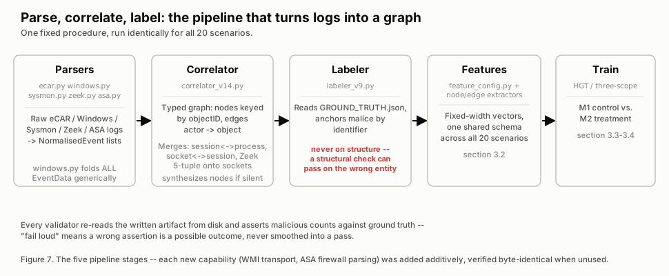 (The data pipeline)
Part 1 ended on a single scenario. Building a study meant going from one to twenty: thirteen attack scenarios built in EvidenceForce (A1-A13), two “failed/contained” scenarios (F1, a firewall-blocked lateral move; F2, a “contained intrusion”), one dual-independent-attacker scenario (D1), and four benign scenarios (B1-B4) 20 total, all built through a repeatable procedure so the process was identical for each scenario. The reason I wanted to include additional scenarios where a SOC identifies and contains a malicious attack chain part way though as well as a scenario featuring dual attackers is so the model does not only get clean training data to learn from. Similarly the benign examples are important so we don’t end up with a model that labels everything as malicious because everything it trained on was malicious.
The procedure was as follows:
- Author the YAML from a scenario spec described above, using only documented storyline event types (
service_installed,scheduled_task_created), because EvidenceForge has nopsexecorschtasksevent type. eforge validate <scenario>.yaml- validate and fix issues as soon as they rear their ugly heads.eforge generate <scenario>.yaml -o <out_dir> -target defaultHere we produces the deterministic log set. Also runeforge evalagainst four hard quality gates (spec conformance, value plausibility, causal ordering, event presence) any issues and it gets sent back to step 1 to iterate.- Inspect the RAW output against the spec, before any pipeline code touches it. Read
GROUND_TRUTH.jsonas the oracle, then confirm each storyline step actually produced the expected records in the expected shape. This is where divergences between “what the spec asked for” and “what the engine actually emitted” get caught and analysed and potentially re-authored. - Run and adapt the pipeline (parse -> correlate -> label) each step validated against the scenario output.
- Verify the built graph against ground truth entity-by-entity ensure timestamps are present and ordered.
- Record and close the loop Document scenario created successfully with any required changes.
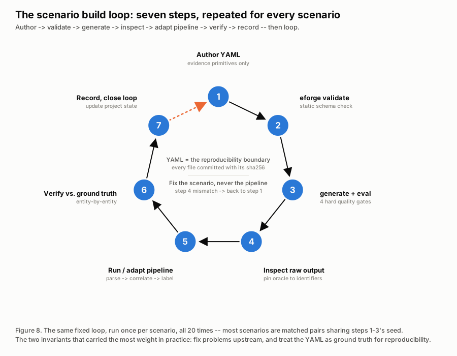 (Scenario Build Loop)
EvidenceForge’s scenario-authoring layer is LLM-assisted and therefore non-deterministic, but generation from a finished, committed YAML is fully deterministic and seeded from scenario.name.
The matched-pair method
Most of the 20 scenarios aren’t just independent data points. They’re actually six matched pairs, each isolating a single axis of variation while holding everything else constant.
Why you may diligently ask? With only 20 scenarios total, an unpaired comparison can’t tell you whether a result reflects the thing you actually changed (transport, dwell time, persistence mechanism, OS) or just incidental differences between two unrelated scenarios. By sharing EvidenceForge’s RNG seed and changing exactly one axis, a matched pair isolates that one variable against an identical background. So when scope 2 catches both A1 (SMB) and A2 (WMI) equally, there we have the evidence that the model generalizes to “crossed a trust boundary”! Rather than just overfitting to one lateral-movement technique’s specific fingerprint.
- A1/A2 (lateral movement): SMB vs WMI transport
- A3/A4 (credential access): LSASS dump vs DCSync
- A5/A6 (persistence): service creation vs registry Run-key
- A7/A8 (dwell time): ~12 minutes vs ~7 hours
- A9/A10 (background noise): low-noise vs ~12x background volume
- A11/A12 (operating system): Windows lateral vs Linux pivot
The method that makes this work is EvidenceForge seeding its run RNG from the scenario’s own name: field. Two YAML files that share the same name and differ in exactly one field will generate identical background activity and identical malicious object identities, diverging only where the deliberately changed field takes effect. A2’s YAML is byte-for-byte identical to A1’s except for one line:
# scenario_a1.yaml
name: a1-smb-lateral
...
storyline:
  - step: remote_logon
    event: logon
    # network_transport defaults to "auto" == stock SMB behaviour

# scenario_a2.yaml - SAME name, ONE field different
name: a1-smb-lateral   # <- shared seed, not "a2-..."
...
storyline:
  - step: remote_logon
    event: logon
    network_transport: wmi   # the only diff: DCOM/RPC 135 instead of SMB 445
Due to some issues which I won’t get into the details, not every pair is this closely aligned. But they’re close enough to meet our goal to be able to compare them.
Where EvidenceForge itself had to be extended
Two of the six pairs needed a capability stock EvidenceForge 1.9.0 didn’t have. Rather than give up on them we created an additive local fork patch.
WMI transport (A1/A2). Stock EvidenceForge’s remote admin storyline bundle is SMB-only. There’s no way to author a WMI/DCOM lateral move at all. The patch adds one field, network_transport: "auto"|"smb"|"wmi", to the storyline logon event; wmi routes a type-3 logon’s establishing cross host connection to DCOM/RPC (port 135, dce_rpc) instead of SMB (445). The edits spanned the scenario model, the auth-session action, the activity generator, and the storyline engine and auto (the default) reproduces stock behavior exactly.
Registry persistence (A5/A6). EvidenceForge has no Reg run key persistence event the stock path is unfortunately a 50% probability, EDR-pool-random registry side effect, which means an authored Run key persistence step was never reliably emitted. The patch hooks the process generator: when a storyline reg.exe process runs reg add <Run-key> [/v <value>] [/d <data>], it now deterministically emits one registry_modify event to that exact key, stamped with the process’s own actor ID - and skips the stock random side effect for that process only. Our existing correlator picks this up through its existing generic actor-to-object path; no correlator change was needed! Only the labeler needed a new rule (rule 3b, scoped specifically to CurrentVersion\Run targets, so an incidental malicious registry write event elsewhere such as A3’s Office key touch correctly stays unlabeled).
F1: when the correlator has to synthesize a node from nothing
Scenario F1 (firewall-blocked lateral movement) forced a different kind of extension. A connection blocked by a firewall produces no eCAR FLOW record at all on the source host. Only the Zeek sensor (a REJ connection state, on the source segment) and a new ASA syslog parser (ported from EvidenceForge’s own MIT-licensed reference implementation) see the events at all. That meant the correlator had to learn to synthesize a socket node when the graph would otherwise have no node to hang a label on. Normally we’d expect to see something in a SIEM from a table like Microsoft’s DeviceNetworkEvents:
def build_asa_deny_nodes(self, zeek_events) -> None:
    """For each retained ASA 106023 deny, ensure a socket node exists
    at its 5-tuple identity - even when eCAR is silent. Resolution
    order: (1) an eCAR-built socket at this 5-tuple, if one exists;
    (2) else a Zeek conn record at the same 5-tuple, synthesize from
    Zeek fields; (3) else synthesize a BARE socket from the ASA
    record's own 5-tuple alone."""
That node deliberately carries no actor edge. Nothing in the graph links any process or session to it, because the only candidate (a Windows 5156 filtering-platform event) is attributed to the generic “System” PID 4 shared by all network activity on the host, a useless anchor. Building machinery to wire that up was considered and explicitly declined as disproportionate in this project. This among some other examples do show how utilising synthetic data has serious downsides compared to real enterprise datasets. But conversely generating dozens or more datasets of actual attack scenarios from a real enterprise SIEM would have it’s own significant challenges. As with everything in life it’s a bit of give and take. My thought process all along this project is if we could get statistically significant results then theoretically the model should hold up against real data.
Feature engineering
Why this is harder than it sounds
A graph node like “the process pd.exe opened LSASS at 14:32:07” means nothing to a neural network until it becomes a vector of numbers. Turning “what happened on a compromised machine” into numbers a model can compare across twenty different attacks, on different hosts, with different personas and different background noise is the actual work of this stage. It’s also a bit more complicated than simply turning a scenario’s own logs into numbers.
(Feature Engineering)
The script feature_config.py created one fixed global schema for all 9 node types (process, socket, session, file, service, registry, module, account, scheduled_task) and all 16 edge/relation types, shared by every one of the 20 scenarios. Each node type gets a fixed-width feature block: one-hot encodings over static, hand crafted vocabularies (hostnames, origins, Zeek service names), multi-hot encodings for things like “which merge stages enriched this node,” and scalar structural features (in-degree, out-degree, total degree, and per-edge-type degree breakdowns). Every node and every edge in every scenario’s graph gets a stable index which is globally shared, This allows the three differently scoped GNNs agree on which embedding belongs to which entity.
One schema decision worth calling out: usernames and persona names are deliberately NOT features. Only structural and derived values go into the tensors. This matters because personas rotate across scenarios specifically so that no single name is consistently “the attacker”. If a name leaked into the feature vector, the model could trivially learn:
“this specific username = malicious,” which would be a shortcut that says nothing about the general provenance-graph thesis.
Obviously in a real detection programme this would be re-considered. However the issue still holds that if the model generated a False Positive for a user account there is a risk all activities from that user would be treated as malicious. There is likely a lot more thought that would need to go into this approach.
Quick explainer on One-hot and multi-hot encoding
As clever as they may be a neural network can’t read the string “sysmon” or “SRV-FILE-01”. Everything, much like our place the the world has to become a number. One-hot encoding is the ML equivalent of normalizing a free-text field into a fixed set of yes/no flags: instead of a string column origin: sysmon, you get a set of columns [origin_ecar, origin_windows, origin_sysmon, ...] with exactly one flipped to 1.
It’s the same concept behind mapping raw vendor-specific alert names onto MITRE ATT&CK technique IDs, so a correlation rule can compare “did this happen” across sources that describe the same thing differently. Multi-hot is the same idea but allows more than one flag on at once. This is used here for “which sensors saw this entity” (a node can be enriched by both eCAR and Sysmon simultaneously, so both flags get set).
The “abused node” concept (9C)
One label-design decision to call out is. A node can be benign (node label 0) while still being the target of a malicious edge. A3’s LSASS process is a real, legitimate Windows process. It did nothing wrong by existing, but the edge representing an attacker’s process opening it with 0x1FFFFF access is malicious. The project tracks this explicitly as an abused metadata flag: a benign node with at least one malicious incident edge. It’s the concept that makes A3’s LSASS and A4’s krbtgt account symmetric rather than looking like two unrelated one off decisions.
Round 3’s feature-layer additions: os and log1p
Two later, smaller feature-layer changes are worth mentioning here:
An os=windows|linux|unknown node feature, added per-hostname by
checking which sensor artifact files actually exist for that host.
row.update(_onehot(hostname_os.get(node.hostname), fc.OS_VOCAB, "os_",
                    other_slot="unknown"))
This mattered for A12 (the one Linux pivot scenario) is otherwise indistinguishable from a Windows host at the structural level except through is_cross_host and the flow bridge an explicit OS signal was found to be a gap.
The three-scope architecture
Part 1’s thesis was that attack signal lives in causal chains spanning log sources rather than in any single event taken in isolation. A single whole-graph GNN sees that whole chain in one pass, which sounds like an advantage, but it also means every node’s representation gets diluted by attention over the entire graph, including tens of thousands of irrelevant benign nodes on a large scenario like A10 or D1. The bet: giving the model three deliberately different fields of view over the same graph one tight and local, one narrow and targeted, one as wide as M1’s own control. Then finally combining their verdicts, recovers signal that gets averaged away under a single unrestricted view.
Scope 1 - process-subtree
Scope one is seeded on every process node, restricted to process lineage relation types only (parent/child creation, and the file/registry/socket edges hanging directly off that process’s own subtree), with a shallow hop budget. Structurally, this is the same as a SOC analyst pulling up one process’s ancestry tree in an EDR console.
This is also where R-CAID’s framing is directly relevant (root-cause localization within a provenance graph, rather than a single whole-graph verdict). Scope 1 is this project’s own analogue of that same idea, built as one input among three rather than the whole system.
Scope 2 - cross-domain-boundary
Scope two is seeded specifically on entities and edges where is_cross_host=1. A structural feature already in the schema, not anything scenario-specific. Lateral movement lights this feature up regardless of which technique caused it (SMB, WMI, RDP all set the same flag), which is exactly why the PAIR-LATERAL matched pair (A1/SMB vs. A2/WMI) exists: if scope 2 only worked for one transport, it would be overfit to a technique rather than to the boundary-crossing structure itself. This would be analogous to the SOC checking for connections from a compromised host during an investigation.
Scope 3 - maximal-context
Scope three has the widest supported “fanout”, no relation-type restriction structurally the same encoder family as M1’s control, but now one of three inputs rather than the only one. The is the hardest aspect of manual investigations casting a wide net on activity can easily lead to rabbit holes and in some cases threat actors generating events purposely to distract analysts. This could be analogous to the SOC checking an hour period before and after the alert for other suspicious events.
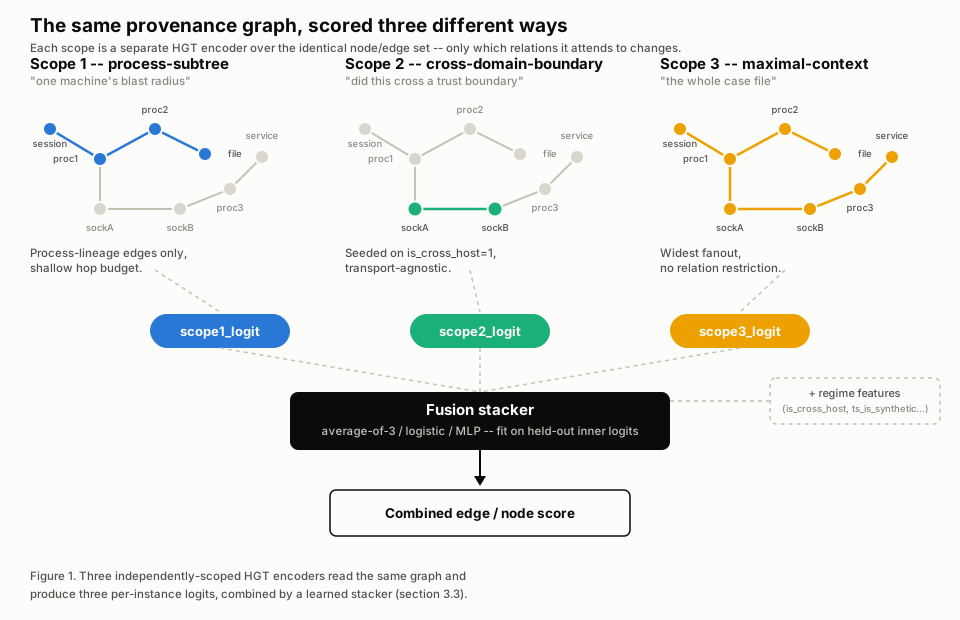 (Three Scoped GNNs)
Why fuse three verdicts?
Different scopes are expected to win on different scenario shapes. A fixed choice of scope would mean picking a single trade off point and living with it across every scenario shape in the study, from a single host LSASS dump to a 70,000-node noisy background to a two-attacker D1. A combination of these scopes could in principle do better than any one fixed view.
Fusion is a small stacker (logistic regression, with an MLP (Multi Layer Perceptron) tried as an ablation arm) over {scope1_logit, scope2_logit, scope3_logit, regime features}, fit with explicit anti-leakage discipline. We built an inner held out subset of each fold’s training scenarios generates the out of sample logits the stacker is actually fit on, so it can never simply learn to trust whichever scope happened to overfit hardest on data it had already seen.
One finding worth flagging:
A directly comparable paper in this same problem space, PROVFUSION (arXiv:2604.14685), reports that simple voting-based fusion of multiple provenance-graph views beats a learned stacker across nine benchmark datasets. A result this project’s own Round 2 work tested against its own data, and which came back with rather mixed results.. More on that later!
Logits, stackers, and fusion
A “logit” is just a raw, unbounded confidence score before it gets squashed into a 0-100% probability. Try to think of it as a raw risk score from a single detection engine before it’s normalized into your SIEM’s severity scale. “Fusion” (via a “stacker”) is the modeling equivalent of a correlation layer that takes several different detection engines’ outputs. For example an EDR score, a network IDS score, and a UEBA score which then combines them into one verdict. Sometimes that combination is a simple average; sometimes it’s a smarter, trained weighting (a “stacker,” here tried as both logistic regression and a small neural network/MLP).
One of this project’s more interesting findings: the simple average beat the “smarter” trained combiner on edge-level detection. A result that will feel familiar to anyone who’s watched a hand-tuned rule outperform a more complex ML-based alert-triage layer in practice.
The model doing the seeing: HGTConv
A Heterogeneous Graph Transformer (HGTConv in PyTorch Geometric) is a transformer-style attention mechanism that is “type-aware” - a login node attends differently to a neighboring process node than to a neighboring socket node, using separate learned weights for each (source-type, relation-type, destination-type) combination, instead of just treating every edge in the graph as interchangeable the way a plain GNN would.
It was chosen specifically because it preserves per-node-type and per-edge-type semantics through attention rather than collapsing everything to one generic type, which matters here because the schema’s 9 node types and 16 edge relations (dc_replication, scheduled_task_create, session_installs_service, and so on).
Attention, and why “type-aware” is the important part
“Attention” is the mechanism a GNN uses to decide how much weight to give each neighbor when forming a node’s updated representation, not every connected event should count equally. That maps directly onto something an analyst does instinctively: When reconstructing a timeline, a parent-child process relationship gets weighted far more heavily than two processes that just happen to share a host at the same time. “Type-aware” means the model doesn’t apply that same weighting logic to a socket connection as it does to a registry write. It learns separate attention weights per (source-type, relation-type, destination-type) combination.
That’s the modeling equivalent of a correlation rule that treats a DNS query and a process-injection event as different categories of evidence, rather than lumping every log line into one undifferentiated stream. Neat.
Model build, test, and validation
The 4-fold split
In machine learning, a fold split refers to randomly dividing a dataset into multiple subsets called folds. This is done to systematically train and evaluate a model. Instead of relying on a single train-test split (which can accidentally give you an overly optimistic or pessimistic evaluation score), a fold split ensures every single data point gets used for both training and testing across multiple iterations. Besides other things this does a good job of maximizing the data usage.
A 4-fold scenario-level rotation was chosen, one benign scenario anchoring each fold:
Fold 1 test: B1, A10, A2, A4, A6
Fold 2 test: B2, A1, A3, A5, A9
Fold 3 test: B3, D1, A8, A12, F2
Fold 4 test: B4, A7, A11, F1, A13
We Verified all 20 scenarios appear in exactly one fold’s test set; all six matched pairs land in different folds so whenever either arm is held out, its partner is in that fold’s training set. Every fold’s test set contains exactly one benign anchor and at least one attack scenario; the three largest graphs (A10, D1, B2) land in three different folds rather than stacking them together.
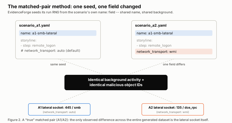 (Matched Pair Scenarios)
Keep this in mind for later: keeping each pair’s partner in the training fold makes this a fair test of “does the axis generalize,” but a soft test of “can the model handle an attack family it has never seen”. Phase 3 (the final section) re-runs the whole thing with families kept together instead, so a held-out fold is genuinely unseen.
The M0-M4 build sequence
- M0 - sampling-equivalence gate. Before trusting any sampled training run, prove that sampled and full batch forward passes on a frozen model produce matching logits. Run first on F2 (smallest scenario with real malicious labels. The smaller B1 has zero positives, making its AUPRC degenerate and useless for this check).
- M1 - single-GNN control. One HGTConv encoder over the whole graph, shared weights across all 20 scenarios, trained/evaluated on the 4-fold rotation. M1 acts as baseline the whole three scope thesis has to beat.
- M2 - three-scope treatment + fusion stacker. The architecture Part 1 proposed, now fully specified: scope 1 (process-subtree, shallow fanout, process-lineage relations only), scope 2 (cross-domain-boundary, seeded on boundary-spanning entities where
is_cross_host=1), scope 3 (maximal-context, widest supported fanout). All three loaders run against the full node/edge set, so every scope produces a prediction for every node and edge, aligned via the same global index. Fusion: a small stacker (logistic regression, upgraded to an MLP as an ablation arm) over{scope1_logit, scope2_logit, scope3_logit, regime features}, fit with anti-leakage discipline - an inner held-out subset of each fold’s training scenarios generates the out-of-sample logits the stacker is actually fit on, so it can’t just learn to trust whichever scope overfit hardest. - M2.5 - a UNICORN-style whole-graph A/B. A lightweight Weisfeiler-Lehman structural sketch (not a full re-implementation of the NDSS 2020 paper just an appropriate analogue) plus a supervised classifier, reduced to the same graph-level grain as M1/M2 via top-k-mean of edge logits. M2.5 was built to answer a separate question: does node/edge-level localization actually buy anything over a whole-graph verdict?
- M3 - temporal message passing. A TGN-style persistent memory scope, fused as a fourth input to the same stacker, gated specifically on the scenarios most likely to need real time-ordering: the dwell pair (A7/A8) and D1 (two independent attackers interleaved in time on one shared identity).
Round 1 results
What AUPRC actually measures?
AUPRC or (Area Under the Precision-Recall Curve) to it’s friends summarizes, across every possible alert threshold at once, the tradeoff between precision (of the things you flagged, what fraction were actually malicious) and recall (of the things that were actually malicious, what fraction did you flag).
It’s the best metric here specifically because of the class imbalance this project keeps running into: in these graphs, malicious nodes and edges are routinely under 0.3% of the total, so a metric like plain accuracy would report 99.7% by predicting “benign” for everything and be worthless. In other words Enterprise logs are noisy malicious events during a compromise account for a tiny fraction of the overall data ingested into a SIEM.
Precision, recall, and AUPRC
Precision and recall aren’t new ideas to anyone who’s tuned a detection rule. Precision in ML is “of everything my rule fired on, how much was actually a True Positive”, and recall is “of everything actually malicious, how much did my detections actually catch”. AUPRC is a single number that summarizes that entire tradeoff across every possible alert threshold at once, rather than at the one specific sensitivity you’d actually deploy at.
That makes it a good tool for comparing two whole architectures, however as this project found the in the “Translating AUPRC” section further down. In some cases it can genuinely hide which one you’d actually want running in production at the threshold you’d pick.
The results
Comparing M1 (single whole-graph GNN) against M2 (three-scope treatment + fusion stacker):
| system | edge_auprc mean (range) | node_auprc mean (range) |
|---|---|---|
| M1 control | 0.1005 (0.03-0.17) | 0.1832 (0.12-0.25) |
| M2 average-of-3-scopes | 0.5755 | 0.3224 |
| M2 MLP stacker (best node arm) | 0.4791 | 0.3660 |
As to suprise no one as I spoiled it at the start The central thesis held, cleanly, in every fold with roughly a 5.7x margin on edge level AUPRC. This ended up being the single strongest, result in the whole study to date. In plain terms: given the same graph, the same features, and the same training budget, three GNNs looking at the same data through different windows and combined by a simple average substantially outperformed one GNN looking at everything everywhere all at once.
One potential surprise however was that simple Averaging beat learned fusion, for edges. The ablation table (control vs. naive average-of-3 vs. logistic stacker vs. MLP stacker) found that for edge level prediction, plain averaging (0.5755) beat both the logistic stacker (0.5487) and the MLP stacker (0.4791). KISS (Keep it Simple Stupid, not the band) showing up as always.
This flew in the face of my naive assumption that a learned combination should always beat a fixed one. In contrast for node-level prediction the opposite held: the MLP stacker was the best arm. The two tasks disagreed on which fusion strategy won, which turned out to be an early sign of the per-fold volatility which the later Round 2 changes attempted to reduce.
The three-scope approach fixes structural complexity, but not scale, or so it seemed at the time. A per scenario breakdown answered the question from M1, “why are D1 and A10 the weakest scenarios”, with what seemed like a sharper distinction than “M2 helps on hard scenarios”. D1 improved dramatically under M2, edge_auprc 0.020 (M1) to 0.455 (average-of-3), ensemble synergy that beat every individual scope. A10 (same attack as A9, but with ~12x the background noise: a scale problem, rather than a structure problem) did not improve: average of 3 (0.049) was actually worse than M1’s own control (0.088) there, with the maximal context scope scoring a near-useless 0.007 on its own.
I opened this whole section with: the widest scope drowns in noise volume, so three-scope fixes structure but not scale.
That conclusion was wrong, and how it was wrong is more useful than the finding it replaced. Those numbers came from an early iteration, before a fix that landed later in Round 1 - and the thing being fixed was that the model’s confidence scaled with how busy a graph was rather than how malicious it was. A10 is the busiest attack graph in the study, ~12x A9.
So the one scenario singled out as M2’s failure case was precisely the one that flaw hit hardest: the breakdown was measuring the bug, not the architecture.
Re-running the same breakdown on the Round 3 models reverses it outright:
| A10, edge_auprc | M1 control | M2 average-of-3 |
|---|---|---|
| early iteration (pre-fix - the artifact) | 0.088 | 0.049 |
| Round 3 (iterations 20/21) | 0.7843 | 0.9565 |
The maximal-context scope that supposedly drowned at 0.007 now scores 0.6677 there, and adds value to the ensemble rather than dragging it down. Measured on the current models, M2’s improvement on A10 (+0.172) is in fact larger than its improvement on D1 (+0.097) - the exact opposite of the original reading, and on both halves of it, since D1’s old numbers came from the same corrupted generation.
Does node edge localization beat a cheap whole-graph detector?
M2.5 compared M1 and M2 (reduced to one graph-level score per scenario) against a cheap Weisfeiler-Lehman structural sketch baseline, on graph-level AUROC. Round 1’s result was mixed/negative: the cheap sketch (AUROC 0.7969) beat both of the project’s own systems (M1: 0.5625, M2: 0.7344). Digging into this found it was almost entirely one scenario’s fault: B2, deliberately constructed “hard negative” (busy, suspicious-looking, but entirely benign activity). Excluding B2 alone, M2’s AUROC jumped to 0.9792. This appears it was likely due to the fragility of a crude top-k-mean graph level reduction against one adversarially hard benign graph. More work needs to be done to make the model less fragile to benign but suspicious looking activity.
Round 2 - Further literature reviews
After Round 1 closed, a second round of literature reviews checked this project’s own empirically found bugs and open threads against published work in the same problem domain.
Interestingly something unexpected popped up during this second lit review. Which shook me to my very core.
To back up slightly this project was first conceived around late march early April. Thats when the initial research and discovery phase brought me to the idea of the three stacked models. Mid April I was very fortunate to take a lovely holiday away which meant I made very little progress besides a bit of studying around GNN’s and the art of the possible. During this time a fantastic paper “Beyond Nodes vs. Edges: A Multi-View Fusion Framework for Provenance-Based Intrusion Detection” apparently came to a similar hypothesis:
“PROVFUSION: a multi- view anomaly fusion and voting-based detection frame- work. To avoid conflating signals, we treat attributes and structure as separate views (details in §4.2). Specifically, PROVFUSION characterizes each system entity from three distinct views: (i) an attribute view that captures deviations in an entity’s intrinsic features, (ii) a structural view that identifies abnormalities in the entity’s role and structure patterns, and (iii) a causal view that evaluates the plau- sibility of interactions (i.e., edges) the entity participates in. We quantify each view independently, fuse them across seven anomaly dimensions, and finalize decisions via a voting-based mechanism, yielding stable performance across heterogeneous score scales.”
The core idea follows the same principal. A single monolithic view of a provenance graph misses signal that a combination of narrower, complementary views recovers. PROVFUSION frames this as “beyond nodes vs. edges” where as this project frames it as “three windows beat one.”
To be clear however, they are quite different in a few ways. This project’s three scopes are the same model looking at three different amounts of the graph. PROVFUSION’s three views are three genuinely different models, each looking at (roughly) the same neighborhood but scoring a different property of it. Whilst we’re both suggesting that looking at three aspects of the graph is better than just a single view, the method is different. I am however very glad of diving back into literature. We’re in such a fast paced world with publications these days that something incredibly relevant can be reviewed and cited within a projects lifecycle.
As an aside as this isn’t an academic research project just a curiosity learning project I do feel very validated that the idea is both novel but is under active research by academic institutions.
Round 3 - pipeline-level changes
Round 3 moved one tier up in cost: changes that require regenerating the stored feature artifacts for all 20 scenarios.
Four items:
os=linux|windowsnode feature;- log1p-scaling the stored degree columns (specifically aimed at closing M2’s still-unresolved logit-magnitude gap);
- Graph-relative normalized timestamp added at the data-loader level (
abs_ts_norm, alongside the existing raw timestamp, non-destructively); - Replacing the old fixed, fold-wide class-imbalance correction with a much gentler, per-scenario, per-epoch negative sub-sampling scheme.
Why “negative sub-sampling” - the class-imbalance problem
In these graphs, well under 1% of nodes and edges are actually malicious. Which in turn means training on every single benign example every round means the overwhelming, normal activity which is the majority of events drowns out the rarer signals. Negative sub-sampling means showing the model a smaller, freshly-resampled slice of the benign examples each training round instead of all of them.
Round 2 + Round 3 results: compared to Round 1
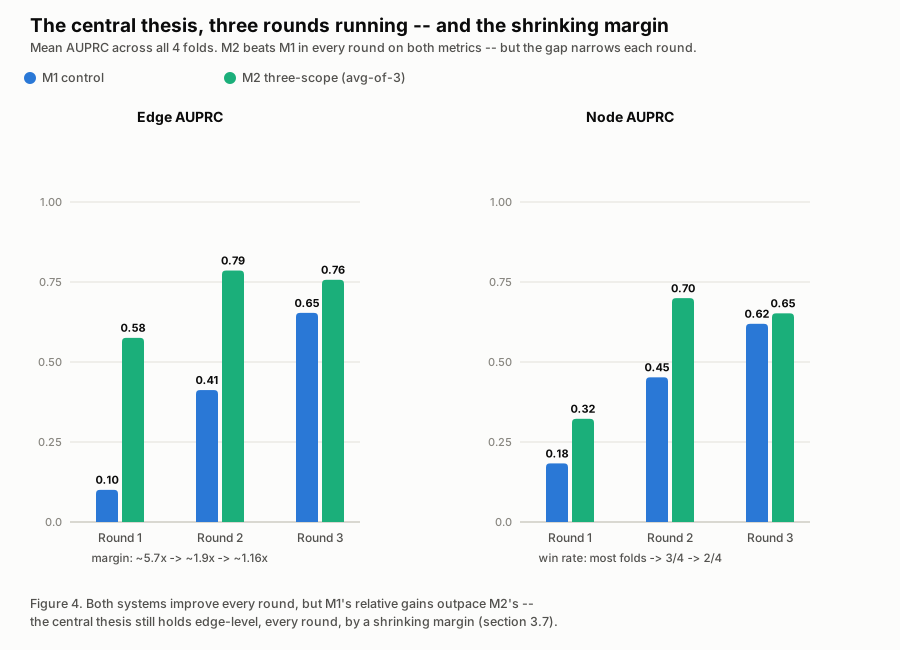
Round 2: a clean architectural win.
| system | Round 1 edge_auprc | Round 2 edge_auprc | Round 1 node_auprc | Round 2 node_auprc |
|---|---|---|---|---|
| M1 control | 0.1005 | 0.4123 (~4.1x) | 0.1832 | 0.4522 (~2.5x) |
| M2 average-of-3 | 0.5755 | 0.7858 (+37%) | 0.3224 | 0.6996 (+117%) |
Good news everyone? The results show every fold improved on both metrics for M1, no exceptions. For M2, every fusion arm improved on both axes except logistic-stacker edge AUPRC, which was flat. The logit-saturation guard (max edge logit under a ~36.0 float64 sigmoid-saturation threshold) improved substantially for M2 - from failing on all 4 folds under Round 1 to failing on 2 of 4 - though it did not fully close.
 (Round based Results)
The central thesis held for the edge-level, on all 4 folds under Round 2’s shared architecture generation. But the margin did narrowed substantially from ~5.7x under Round 1 to ~1.9x under Round 2. This narrowing turned out not to have a simple explanation. M1’s absolute gain (+0.3118 edge_auprc) actually exceeded M2’s (+0.2103). A hypotheses was left open with the available data:
M2 received an extra change (pre-norm placement) that M1 did not, there is the potential that change’s own known stability-vs-peak-performance tradeoff cost M2 some ceiling.
For the Node-level, the picture had one characterized exception: M2 beat M1 on 3 of 4 folds, with fold 2 (which includes B2, the study’s own deliberately hard negative) going the other way, however to be clear this has not been confirmed as the culprit.
A follow-up pass on the same round’s already-saved logits tested two more ideas from the literature review and both came back negative-to-mixed, reported in full rather than smoothed over. Voting/rank fusion (testing PROVFUSION’s finding directly): a naive vote-count arm was the clear worst of five arms tried, because with only 3 scopes it produces just 4 distinct values, which is far too coarse a ranking signal for this domain’s extreme class imbalance; a rank-average arm was respectable but still didn’t beat plain averaging.
PROVFUSION doesn’t vote across three raw view scores the way this arm did. It calibrates a set of separate threshold detectors built from those scores: single-view, pairs, and all-three. Then it takes a majority vote across all of those. So this arm tested the general intuition that voting might beat averaging, and found that it didn’t here.
A larger stacker-fit subset (8 scenarios instead of 4). It helped the logistic stacker broadly, but hurt the MLP stacker, including one absolutely catastrophic single-fold collapse. Model complexity interacts with fit set size non-uniformly; more data is not a universal fix for stacker instability. Average-of-3 remained the recommended, most stable fusion arm on both axes throughout.
One clean reversal did land: M2.5’s Round 1 finding (“the cheap sketch beats both our systems on graph-level AUROC”) flipped entirely under Round 2. Both M1-reduced and M2-reduced now beat the sketch on both AUPRC and AUROC (M2: AUROC 0.9688 vs. the sketch’s 0.7969).
The deliberate fix built specifically to address the B2-driven fragility behind the Round 1 result (a median-of-top-k reduction, meant to be more robust to one outlier high-confidence false-positive edge) turned out to be unnecessary and was itself rejected the results being uniformly worse than the simple top-k-mean it was meant to replace, most plausibly because Round 2’s other changes had already fixed B2’s specific fragility as a side effect.
The targeted M3 batch-size probe (varying only BATCH_EVENTS, re-training only the temporal scope on D1’s own saved static logits) produced a striking but inconclusive result. At the finest granularity tested (BATCH_EVENTS=20), the temporal scope reversed and actually helped D1 for the first time in the study (delta +0.0404). However the intermediate value (BATCH_EVENTS=50) was the worst of the three values tested (delta -0.0796), which does not fit a simple “smaller batches monotonically reduce staleness” narrative.
Single-seed, single-run at each value. This was found that it cannot separate a real effect from training-run noise, and is flagged as the most promising unexplained thread in the whole probe rather than either adopted or dismissed.
Round 3: M1 improves cleanly; M2’s picture gets more complicated
| metric | Round 1 | Round 2 | Round 3 |
|---|---|---|---|
| M1 edge_auprc mean | 0.1005 | 0.4123 | 0.6535 |
| M1 node_auprc mean | 0.1832 | 0.4522 | 0.6193 |
| M2 edge_auprc mean (avg-of-3) | 0.5755 | 0.7858 | 0.7568 |
| M2 node_auprc mean (avg-of-3) | 0.3224 | 0.6996 | 0.6521 |
| Central thesis (edge) | holds, ~5.7x | holds, ~1.4x-2.5x | holds, ~1.02x-1.29x |
| Central thesis (node) | holds, most folds | 3 of 4 folds | 2 of 4 folds |
| M2 saturation guard (<36.0) | n/a (pre-fix) | 2 of 4 folds exceed | ALL 4 folds exceed |
M1 improved cleanly across the board, every fold, both metrics. The most plausible driver being the new negative-subsampling scheme. A ~20:1 ratio replacing the old 878x-3119x fixed pos_weight, a roughly two-orders-of- magnitude gentler imbalance correction.
M2’s picture is… mixed:
- Edge-level, the central thesis still holds on all 4 folds M2 beats M1 in every fold. But the margin narrowed again, past Round 2’s own narrowing: from ~5.7x (Round 1) to ~1.4x-2.5x (Round 2) to ~1.02x-1.29x (Round 3). Fold 4’s margin, 1.02x, is barely above parity, the smallest edge-level margin recorded anywhere in this study.
- Node-level, the win rate regressed: M2 beat M1 on only 2 of 4 folds (down from Round 2’s 3 of 4). Round 2 had one characterized exception in fold 2. Round 3 adds a second exception (fold 4) with no established cause yet.
- The logit-saturation guard, the exact thing the log1p feature-scaling change was aimed at fixing. This turns out WORSE, not better. Round 2 had 2 of 4 folds exceed the 36.0 threshold; Round 3 has all 4 (36.00-52.41), the worst logit-magnitude result recorded for M2 in the entire study. The negative subsampling change, is the most plausible driver, since a far gentler imbalance correction plausibly lets the optimizer reach sharper, higher-magnitude decision boundaries without the old extreme
pos_weight’s implicit damping effect. While there’s no obvious mechanism by which log1p-scaling raw features would increase logit magnitude.
What “logit saturation” means, without the maths
Picture a confidence dial that’s supposed to range smoothly from “not suspicious” to “extremely suspicious.” A bug in this project caused that dial to slam all the way to maximum for almost everything. Benign hosts included, because a handful of badly-scaled features (a raw connection count in the thousands, sitting next to features valued in the tens) blew the model’s internal maths past the point where its output function can still tell scores apart.
Once every score reads “maximum confidence,” you’ve lost the ability to rank anything by how suspicious it actually is. It’s the modeling equivalent of a detection rule that fires at mathe highest severity on both a real incident and routine background noise - technically “detecting” both, but useless for triage.
TLDR
The summary for a reader who wants the state of the central thesis in one sentence: three-scope beats single-scope, edge-level, in every fold, across all three rounds so far. That being said the margin has shrunk each round, and the node-level half of the same claim is the weakest and least settled part of the whole study right now.
Update from Phase 3 (final section of this post): both of those caveats turned out to be Round-3-specific. On the much larger 49-scenario corpus the edge margin did not keep shrinking. In fact it widened back out to roughly 2.8x and the node-level claim, the part called “least settled” above, held cleanly in every fold.
Translating AUPRC
A single AUPRC number, doesn’t answer the question a SOC analyst actually has: “if I deployed this, what would my alert queue look like?” Precision at fixed recall, computed directly from the real held-out predictions (pooled across all 4 folds - all 20 scenarios, each scored out-of-sample exactly once), answers that more concretely:
Edge-level (241,553 pooled edges, 242 positives, base rate 0.10%):
| recall | M1 precision | M2 precision |
|---|---|---|
| 50% | 71.2% | 85.2% (M2 ahead) |
| 70% | 56.9% | 59.4% (M2 ahead, slim) |
| 80% | 39.4% | 49.6% (M2 ahead) |
| 90% | 22.8% | 9.4% (M1 ahead) |
| 95% | 10.1% | 3.1% (M1 ahead) |
This is a somewhat counterintuitive finding: M1 has better precision than M2 at 90-95% recall, despite M2’s much higher overall AUPRC. AUPRC integrates over the whole curve and rewards M2’s substantially stronger middle band even though M1 wins the tail. In practical terms: if the deployment goal is “keep the analyst’s review queue clean, catch most things,” M2 is the clear win. If the goal is “catch nearly everything, and accept the noise that comes with it,” M1 is not obviously the worse choice, despite its much lower headline number a nuance the single AUPRC figure hides completely.
A separate, more reassuring check: for every attack scenario, how deep would a SOC reviewing one combined, pooled queue have to go before that incident’s first real alert appears? Both models surface nearly every incident (worst non-outlier case: M1 rank 55, M2 rank 26, out of ~241,000 pooled edges). F2 - the deliberately subtle, contained-before-lateral-movement scenario - is a hard outlier for both models (ranks 740 and 207 respectively), which is arguably the expected, not the alarming, result: F2 was built specifically to be the hardest case in the study. The practical reading: the three-scope treatment’s real value-add isn’t “catches incidents the single-GNN control misses entirely” - both catch nearly everything. The real advantage is the cleaner mid-recall queue shown in the precision table above.
Detect, then reconstruct?
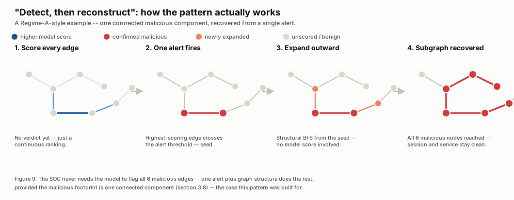
A recurring pattern in published provenance-graph intrusion detection (KAIROS, ORTHRUS, and similar systems) is “detect, then reconstruct”: don’t try to score every node and edge with equal confidence - catch one suspicious anomaly, then use graph structure to walk outward from it and recover the rest of the causal chain.
 (Detect Then Reconstruct)
If we think about it this maps naturally onto how a SOC actually works: an analyst doesn’t need the model to flag all thirteen malicious edges in an incident, they need one alert to trigger an investigation, after which normal incident-response process (following identifiers, pivoting on hosts and sessions) does the rest.
Step 1: does at least one alert fire?
Yes, almost always, for both models, covered above in the first-alert-rank table. Whilst I am repeating myself here it’s important to note it’s the necessary precondition for everything that follows: if the first alert never fires, there’s nothing to expand from.
Step 2: does one alert’s neighborhood recover the entire malicious subgraph?
Structural BFS
Breadth-first search (BFS) here just means: starting from one flagged edge, walk outward to its directly connected nodes, then their neighbors, and so on, adding each new node to the “recovered” set as you reach it. This is the automated version of exactly what an IR analyst does by hand when they pivot from one IOC to related hosts, accounts, and processes in a SIEM or EDR console. The question this project is really asking is: if the model gives you one solid starting point, does that manual-pivoting process get you the rest of the incident for free?
Essentially no, when seeding from each scenario’s own single highest-scoring true-positive edge, and doing a pure structural breadth-first search outward over the observed graph only the scenario F2 reaches 100% coverage from a single seed. Every other scenario plateaus well short of full coverage.
A4 makes a good case study for why. Direct inspection of its malicious-adjacent edges shows its 7 malicious nodes split into 5 structurally disjoint clusters.
The DCSync process and its immediate neighbors form one cluster; a session/process/socket/service hub forms a second; a second, entirely separate session forms a third; and two individual nodes are isolated, their only edges leading to non-malicious neighbors.
The root cause:
EvidenceForge mints a fresh session or process identity per anchoring event, rather than reusing one identity across a whole authored narrative, so what an analyst would naturally call “one attacker session” can show up as two or three entirely separate graph nodes with no edge connecting them, even within a single scenario’s own ground truth. This is the identical mechanism already documented for D1’s two independent attackers sharing one compromised identity shown to occur within one attack’s own footprint.
Step 3: Seeding from the model’s own top-K alerts
The single-seed BFS is a useful diagnostic, but it’s not how a SOC actually works: a real alert queue mixes true and false positives, and an analyst expands from however many alerts the top of the queue actually contains, not from a hand-picked perfect seed. Re-running the same expansion from the top-K ranked edges (true or false positive, K increasing from 1) and finding the smallest K at which BFS recovers the full malicious node set produces a bimodal result:
- 8 of 16 attack scenarios converge at K=1-3, at 100% precision - every seed alert used is a real true positive, zero false-positive budget spent. These are the scenarios where the malicious footprint is already one tight structural cluster.
- 6 of 16 converge only at K=41-69, with precision collapsed to 24-64% - dozens of false-positive alerts have to be absorbed before one happens to land near the missing structural island.
- 2 of 16 (A12, F1) never converge even at K=80.
The most critical finding here: whether seed-and-expand works at all and is it predictable from graph structure, not just from model confidence. The scenarios that fail don’t fail because the model scored them poorly. Many of the “Regime B” scenarios’ true positives are ranked well inside the top 20. They fail because the ground-truth malicious footprint itself is structurally fragmented, so no amount of additional high-confidence alerts helps once every already-connected cluster’s own alerts are exhausted. In this instance only a coincidental false positive landing near the missing island bridges the gap.
Next Steps
I still have a laundry list of things I want to do with this project. The three major ones are:
- Build a lot more varied scenarios,
- More deeply explore the possibilities and capabilities behind the idea of detect then reconstruct
- Work out how the data pipeline could be migrated to ingest real world datasets rather than being tied to EvidenceForge output
My plan was a two part project but largely because i’ve been enjoying ths process of learning and exploring so much I want to continue to improve and iterate and expand the capabilities. I’m delighted that my core hypothesis was confirmed although either result would have been educational and I am also happy a second round of literature reviews show academic research as recently as April (after this project started) is also exploring a very similar 3 scope PIDS idea.
…and, as it happens, the first of those three objectives: “build a lot more varied scenarios” is what I went and did next, along with a full retrain on top of it. So Part 2 doesn’t quite end here after all, more writing for me, reading for you. Apologies not quite there yet.
Phase 3 - A new set of scenarios and the results
Part 2 was meant to stop at that Next Steps list. Then whilst procrastinating writing this behemoth up I kind of accidentily carried on with the project and completed the first of my planned Phase 3 objectives. A big round of new scenario generation that roughly doubled the dataset, a deliberately large “enterprise” scenario, and a final retrain that put the whole thesis through its hardest test yet.
The one-line version: the thesis didn’t just survive this new harder test, it came through it more convincingly than at any point in Part 2!
From twenty to forty-nine
The single biggest weakness of the Part 2 study was breadth. Twenty scenarios, six attack families. A skeptical reader (myself included) could reasonably ask whether “three windows beat one” was a real property or an artifact of the specific handful of attacks I just so happened to build. So the goal for this round was a lot more more variety. Wspecially attack stages the original twenty never touched (command-and-control, exfiltration, initial access, defense evasion). Add into the mix enough benign hard-negatives alongside them that the model can’t cheat by learning “this technique’s tools = bad.”
The corpus went from 20 to 49 scenarios. The new arrivals, which are grouped by what they were for:
| Scenario(s) | What it is | Why it earned a place |
|---|---|---|
| a14 / a15 / a16 | Noise-volume sweep - the same small attack buried in progressively busier graphs (14k, 32k, 141k nodes) | Fill the gap between the original quiet point (a9, ~6k nodes) and noisy one (a10, ~70k), plus an extra-large one, so “does the wide scope drown in noise” can be answered across a controlled scale sweep instead of a single data point |
| e1 / e2 | C2 beacon vs DNS-tunnel exfiltration | A whole attack STAGE the original 20 never covered - command-and-control and data egress. Axis = the egress channel |
| s1 / s2 | Credential spray that succeeds vs one contained before it does | Password spray is one of the most common real-world initial-access techniques and had zero representation |
| s3 / s4 | Spray (one password, many accounts) vs brute-force (many passwords, one account) | Same outcome, opposite shape - a clean test of whether the model keys on the attack pattern |
| s5 / s6 | Spray from an external internet IP vs from an already-compromised internal host | Source axis - does the model care where the spray originates |
| l1 / l2 | Living-off-the-land (System32 built-ins) vs a dropped, named tool | The fileless-vs-dropped-binary distinction every detection engineer knows matters |
| k1 / k2 | Kerberoasting, targeted vs mass | A classic Active Directory credential technique - and it forced a brand-new edge type into the schema |
| g1 / g2 | Group-membership privilege escalation, used vs dormant | T1098; added an entirely new node type (a security group) |
| i1 / i2 | Insider threat, business hours vs after hours | The study’s FIRST no-compromise attack: a legitimate user, own session, no malware, no exploit - malice is the pattern and the timing. This one becomes the interesting counterexample later |
| p1 | Phishing delivery -> foothold | One of only two INITIAL-ACCESS scenarios; everything before it started post-compromise |
| x1 | External remote services (stolen creds -> external RDP -> fileless foothold) | The other initial-access case, and the hardest to signature - no malware at all |
| v1 / v2 | EDR disablement vs Windows event-log clearing | Defense evasion (MITRE TA0005), a whole tactic the original 20 skipped |
| y1 / y2 | Bring-your-own-vulnerable-driver, persistent vs load-then-unload | Kernel-driver abuse, another gap in coverage |
| b5 / b6 / b7 | Three new benign hard-negatives | Specificity controls: a benign admin using the same built-in tools as l1, a benign noisy-DNS host that looks like e2’s tunnel, and a benign auth-failure storm that looks like a spray. So the model learns the difference rather than a shortcut |
| w1 | A ~1 million-node enterprise (its own subsection below) | Does any of this hold at realistic enterprise scale |
These were built the same way as the original twenty. A repeatable and largely reliable author/validate/generate/inspect loop from earlier in this post, creating a the matched-pair wherever an axis could be isolated. In a couple of cases also I ended up with an additive local-fork approach where a technique needed a capability stock EvidenceForge didn’t have (kerberoasting and group-membership each added a new relation or node type to the schema, taking it to 10 node types and 18 relations). As before, some pairs are “true” matched pairs that differ in a single field, and some are partial.
The million-node scenario, and the wall I hit
w1 is the odd one out. Every other scenario is a single incident. Consisting of the one attacker, one chain, a few thousand to a few tens of thousands of nodes. w1 is a deliberately different beast: one enterprise of 993,464 nodes and 905,578 edges (call it ~1.0M), 77 hosts across 6 subnets, 213 users, and 7 completely separate attack campaigns running concurrently (SMB lateral + service, WMI + scheduled task, DCSync, kerberoast, spray, insider, and a C2/DNS-exfil pair), each drawn from the repertoire above. This was designed as a stress test: does the pipeline hold, and does the three-scope advantage survive at a scale that looks more like a real network than a single lab incident.
The new folds, and a harder test than Part 2’s
Part 2 evaluated on a 4-fold rotation over 20 scenarios, deliberately putting each matched pair’s two arms in DIFFERENT folds, so whenever one arm was held out for testing, its partner was still in training. Designed to test “does the axis contrast generalize,” and in addition test “can the model handle an attack family it has never seen,” because a near-identical sibling is always present.
For the final Phase 3 result I ran the cross-validation two ways:
- Grouped (the headline). Every scenario that shares an attack family tests together in the same fold. When kerberoast is the held-out fold, NEITHER kerberoast scenario is in training. This is the genuine “unseen family” test.
- Split (the secondary). The old Part 2 arrangement - partner arm always in training. Tests generalization across the controlled axis.
The full 49 got folded into a 7-fold cross-validation (there are exactly 7 benign scenarios, so one anchors each fold, 4 folds with 4 benigns). Two sets of scenarios were pulled out of the rotation entirely and kept as standing benchmarks, scored by every fold’s model but never trained on: the noise-scale trio (a14/a15/a16) and the million-node w1. And for the final number I ran three random seeds instead of one and reported the spread.
“grouped” vs “split” holdout
Think of it as two ways to grade detection coverage. The “split” grade is: you built and tuned a rule against one SMB lateral-movement sample, and I now test it against a different SMB lateral-movement sample in the same environment. The “grouped” grade is harder and more true to the real world: I test your coverage against an entire technique family you have never tuned against at all. The first time this class of attack has crossed your desk. A detection approach that only holds up under “split” grading generalizes across small variations; one that holds up under “grouped” stands a chance against genuinely novel tradecraft. Phase 3 reports both, and leads with the harder one.
- M1 (the single-GNN control): started 00:08, finished 03:13 - 3 hours 5 minutes.
- M2 (PARALLAX, three scopes + fusion): started 03:13, finished 16:19 - 13 hours 6 minutes.
- Total: about 16 hours.
M2 costs roughly 4x M1 because it’s training three encoders plus a fusion layer per fold instead of a single encoder.
The results
A bigger, more varied corpus with genuinely unseen attack families is a much harder test than Part 2’s, and it would have been entirely reasonable for the barely-above-parity margins from Round 3 to collapse to nothing. They didn’t. On the headline (grouped) regime, averaged over three seeds and seven folds:
| M1 control | M2 (PARALLAX) | ratio | |
|---|---|---|---|
| edge AUPRC | 0.2534 | 0.7154 | 2.82x |
| node AUPRC | 0.2904 | 0.5226 | 1.80x |
M2 beat M1 on every single fold, both metrics, in both regimes - 28 out of 28 fold-by-fold comparisons. And the separation isn’t marginal: M2’s WORST fold (edge 0.5352) still beat M1’s BEST fold (0.4202). This is comfortably the strongest result in the whole project, and it’s on the hardest test that was built.
One number needs a caveat: M1’s headline here (0.2534) is a lot lower than the 0.6535 it scored in Part 2’s Round 3. That is NOT M1 getting worse, it’s the test getting much harder (49 scenarios instead of 20, with unseen-family holdout). The only fair comparison is M1 vs M2 on the same footing, and there M2 is 2.82x ahead. Comparing across the two studies would be comparing a harder exam to an easier one.
The two standing benchmarks:
| held-out benchmark | M1 | M2 |
|---|---|---|
| noise-scale (a14/a15/a16) | 0.310 | 0.907 |
| enterprise (w1, ~1M nodes) | 0.160 | 0.541 |
The noise-scale result is the one I find most satisfying, because it’s the direct, at-scale rebuttal to the old “the wide scope drowns in noise” story from Part 2’s Round 1: the same small attack buried in graphs from 14k to 141k nodes, and M2 recovers it almost perfectly (0.907) where the single GNN mostly can’t (0.310). The enterprise w1 is the widest relative margin of all (over 3x), even if the absolute numbers are lower. A million-node, seven-campaign graph is a genuinely hard problem, and honestly I’d have settled for “doesn’t fall over.” And the standing method call from Part 2 held up a fourth time: plain averaging of the three scopes still beat both the learned (logistic and MLP) fusion stackers, across the board.
Focusing on two aspects of the results
The grouped and split came out level (edge 0.7154 vs 0.7225). Looking closer, per-scenario there IS a small, consistent penalty for holding a whole family out. It’s cleanest exactly where I’d expect, on the handful of “true” pairs that share the most malicious structure (all six of those arms scored lower with their partner absent). It’s just small enough that the big, easy, high-volume scenarios wash it out of the pooled average. At ~45 training scenarios, the model has seen enough related attacks that any one family’s specific partner is close to redundant. Meaning the model isn’t simply just leaning on a memorized sibling.
Under the grouped regime, two folds hold out an ENTIRE capability: kerberoasting, and group-membership privesc. The model has to score a technique whose distinctive edge type it literally never saw in training. It still won those folds. It manages this because it recognizes the malicious PROCESS driving the technique (which looks like every other attack’s foothold and recon activity), and the novel edge inherits suspicion from its malicious source. That’s a rather encouraging property for detection: it manages generalise onto techniques it wasn’t trained on, as long as the surrounding chain is familiar.
Second, the counterexample. It turned out there is at least exactly one attack family the whole approach is bad at, the insider threat (i1/i2), and especially the after-hours arm (i2), which the model scores at essentially zero (edge AUPRC 0.006). None of the three scopes see it. A legitimate user, on their own machine, using only built-in Windows tools, collecting files and uploading them over normal HTTPS. There is no structural anomaly. Every process looks like admin work; every connection looks like ordinary web traffic. The ONLY thing separating the malicious activity from the benign background is timing (it happens at 9pm) and intent. These happen to be the attacks traditional detection engineers and SOC’s strugle with the most and so I hope to revist this to see if any improvements can be made. Anyone who’s naievley trued to build an anomaly detection for logins or activity out of hours for anything but the most locked down environments know it’s basically a non starter.
Whilst this boundary of “attack signal lives in causal chains.” i2 IS a causal chain (collect -> stage -> exfiltrate), but a chain made entirely of individually-innocent steps by a trusted user, so structure alone can’t catch it. Digging in, I also found a concrete, fixable contributor: the timestamp feature I’d built specifically to expose exactly this kind of timing signal (a graph-relative normalized time) wasn’t actually being fed into the scope models in this run.. It’s computed and stored, but the models never see it, incompetance on my behalf. So part of i2’s failure is “the model can’t see time,” and part is “the one time feature we have wasn’t plumbed in.”
Where this leaves things?
Phase 3 did what I hoped: it took the central result off the small, tidy 20-scenario bench and put it on a much messier, more realistic 49-scenario one. This was including a million-node enterprise and attack families the model had never seen. Consistently the three-scope approach won more decisively than before! The margin didn’t shrink this time; on the hardest test in the project it widened back out to nearly 3x. The node-level half of the claim, which I flagged in Part 2 as the weakest and least settled, also came through cleanly here, with M2 ahead in every fold.
As for whats next? I need to decide on feasibility of converting this project to work with real life data sources rather than the output of evidence forge. Then ideally release it!
References
- Hu, Z., Dong, Y., Wang, K., Sun, Y. “Heterogeneous Graph Transformer.”
WWW 2020. arXiv:2003.01332 (the model family this project builds on
directly via PyTorch Geometric’s
HGTConv) - Han, X., Pasquier, T., Bates, A., Mickens, J., Seltzer, M. “UNICORN: Runtime Provenance-Based Detector for Advanced Persistent Threats.” NDSS 2020. https://arxiv.org/abs/2001.01525
- Goyal, A., Wang, G., Bates, A. “R-CAID: Embedding Root Cause Analysis within Provenance-based Intrusion Detection.” IEEE S&P 2024. https://gangw.cs.illinois.edu/rcaid-sp24.pdf
- Cheng, Z. et al. “KAIROS: Practical Intrusion Detection and Investigation using Whole-system Provenance.” arXiv:2308.05034
- “ORTHRUS: Achieving High Quality of Attribution in Provenance-based Intrusion Detection Systems.” USENIX Security 2025. tfjmp.org/publications/2025-usenixsec.pdf (also the source for the VELOX comparison, per that same body of work)
- “MAGIC: Detecting Advanced Persistent Threats via Masked Graph Representation Learning.” USENIX Security 2024. arXiv:2310.09831
- “Beyond Nodes vs. Edges: A Multi-View Fusion Framework for Provenance-Based Intrusion Detection” (PROVFUSION). arXiv:2604.14685
- “PIDSMaker: Building and Evaluating Provenance-based Intrusion Detection Systems.” arXiv:2601.22983
- “Are we really making much progress? Revisiting, benchmarking, and refining heterogeneous graph neural networks.” arXiv:2112.14936
- “GRANOLA: Adaptive Normalization for Graph Neural Networks.” arXiv:2404.13344
- EvidenceForge: https://github.com/Cisco-Talos/EvidenceForge