Provenance based Graph Neural Networks using Heterogeneous Graph Transformers

June 16, 2026 • 4460 words • 21 min

Scene Setting

If anyone recalls the first post I wrote back at the end of January I suggested more content might come sooner than half way through the year. Without dwelling on that too much, I would love to introduce the first half of a two part installment. Here we will largely focus on the problem statement, theory, research background followed by the data pipeline I’ve built. Then hopefully this will be able to surface some interesting results in part 2.

The aim of this project is to train a high fidelity detection engine on sequences of suspicious events. Building from logs which are representative of a typical Enterprise SIEM. Which in theory should be portable to any typical SOC environment. Emphasis on the theory.

Framing

Let’s begin with the problem statement.

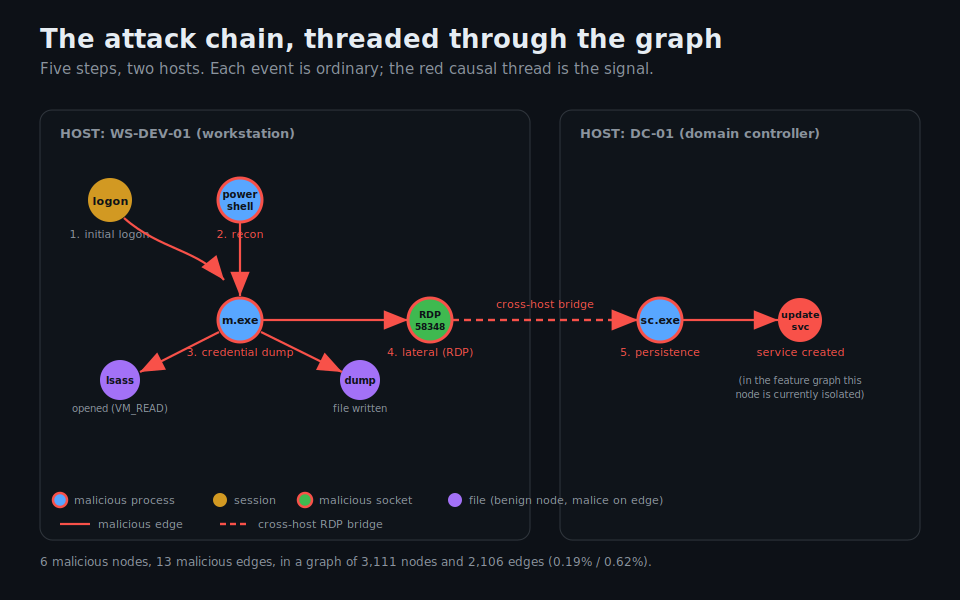
The average compromise or intrusion is often observed as a sequence of small mundane events. An identity logs in and executes a process which spawns a child. That child process reads another process’s memory then opens a network connection. A service gets created.

Each of these, on its own happens thousands of times a day on a normal enterprise network. These activities would likely not trip any rule worth writing. A rule that fires on a process that read another process’s memory would end up firing constantly. And as we know that leads to it being tuned out within a week (or longer depending on the week). Detection engineering is always a delicate knife edge balance. On the other extreme if we only write detections for activity which is unambiguously malicious we’re almost certainly going to miss any sort of subtle attack. On the other we have the noisy scenarios described above.

The aim of good detections is that try to absorb as much context from that single event and only alert on exceptions to the norm. As an example for a sign in event this is the user agent, the location, the time, the IP reputation. But even when taking as much context into account as possible we still have to tread the line between missing the malicious sign in vs alerting off a large amount of benign sign ins.

Not to put too fine a point on it, if you only have fantastic detections that identify clear signs of compromise like ransomware or 2tb of data being exfiltrated. By the time those alerts have fired, the SOC has performed L1 triage and escalated the issue to your Incident Response Team, and a lot of the damage has likely been done. That is to say in an ideal world we want to identify and stop an attack as early in the attack chain as possible but quite often activity early in the lifecycle is more prone to false and benign positives.

Most likely this isn’t news to you. This entire topic has been discussed to death across papers, conference talks and promises given by vendor pitches. Equally attempting to treat the problem with Machine Learning as a panacea is absolutely not novel. EDR vendors in particular have been making heavy use of Machine Learning for many years to varying levels of success. SOC teams often have a hard time, the algorithms may be trained on a 30 day period of logs and then left to their own devices. Unlike traditional Detections where tuning is usually trivial, Machine Learning rules tend to be somewhat opaque beyond a vague description of “Anomalous sign in” and provide little levers to effectively tune.

I have a strong suspicion that a great deal of this challenge stems from the fact that detections be they EDR/SIEM rules or Machine Learning rules—tend to focus on a single category of events. They may focus on a suspicious login (everyone’s favorite Impossible Travel or Risk Sign in), process injection, a malware signature. These events will be grouped together but they still only focus on a single type of event.

Approaches like RBA (Risk Based Alerting) do go a long way to solve this problem through aggregating risk scores for multiple alerts seen against an entity in a rolling time window. They are aggregating individual events into a cumulative score rather than clearly identifying the links between those events. An RBA alert can often comprise 5 or 6 entirely unrelated risk events that happened to occur within that time period.

As we discussed at the outset the “subtle” signals are not necessarily surfaced any of those individual events. The signal we are looking for is expressed in a chain of related events: A login, led to a process being spawned, this process read lsass (the Windows process that holds credentials in memory), which wrote a file, which was carried over this RDP session to that host, which created this service. The malicious activity flows through the causal thread connecting ordinary events across log sources and across machines.

In this series of blog posts want to reframe the entire detection problem to focus on causal chains of activity. TThis still leaves us with the question: how do we find a solution that addresses the problem as we have now framed it? A potential solution is we can build a causal graph and train a model to recognise the malicious subgraph (series of events which were malicious).

This is a graph-learning problem, and that’s where this project starts.

alt text

Research & Provenance

Provenance-based intrusion detection (PIDS) is a well established line of research, and this project leans into it heavily. I’d like to reference a few papers as an introduction, because they set the groundwork and guided my thinking for how I am conducting my approach.

Before delving in, it’s probably useful to offer a definition before throwing out too much technical jargon:

Provenance-based intrusion detection (PIDS) models system activity as a provenance graph. This can be described as a directed graph whose nodes are system entities (processes, files, sockets, users) and whose edges are the interactions between them (a process reading a file, opening another process, connecting to a host). Because the graph captures the causal dependencies between events rather than the events in isolation, an intrusion shows up as an anomalous pattern of interdependencies. Essentially highlighting it as a malicious subgraph. This gives an attack technique agnostic view, you’re not matching known signatures or even individual behaviours, you’re looking for structure in your logs that deviates from benign execution.

UNICORN (Han, Pasquier, Bates, Mickens, Seltzer; NDSS 2020) is the one that framed the problem for me. It’s an anomaly-based APT detector built on whole-system provenance graphs, and it’s explicitly designed around the “low-and-slow” problem. Attacks that unfold over a long enough span that any short window of events looks normal. Its answer is to summarise the entire evolving graph efficiently through a “graph-sketching technique” rather than just inspecting local neighbourhoods. The argument being that the context you need to separate benign from malicious lives in the long causal relationships, not the immediate ones.

R-CAID (Goyal, Wang, Bates; IEEE S&P 2024) highlights a different point that has directly shaped my design. It names the “curse of locality”, when you embed a provenance graph by aggregating local neighbourhoods, you sever the link between a suspicious event and its root cause. R-CAID’s response is to precompute each node’s root causes during graph construction and fold them into the embedding, allowing the model to perform detection at the node/process level rather than classifying a whole graph as malicious or benign.

For the model itself, the family I’m targeting is HGT, the Heterogeneous Graph Transformer, the graph is heterogeneous (not a single type of thing). Processes, files, sockets, sessions are different kinds of nodes with different feature spaces. HGT maintains per-node-type and per-edge-type message-passing semantics instead of flattening everything into a generic type. The whole feature schema I describe later is built around that per-type structure. Most earlier graph neural networks assumed every node was the same kind and every connection meant the same thing, which forces you to flatten that distinction away. HGT keeps it.

It does this by treating each connection as a typed fact: this kind of node, connected by this kind of relationship, to that kind of node. “A process opens a socket” and “a session runs a process” are handled as distinct relationship types with their own learned behaviour, rather than being lumped together.

The “Transformer” part borrows the same core idea that powers large language models: attention. When the network builds up its understanding of a node, it doesn’t treat all the node’s neighbours equally. It’s able to learn which neighbours matter most for the task and weights them accordingly. So a process surrounded by ten ordinary children and one connection to a credential store can learn to pay disproportionate attention to that one unusual connection. Attention is what lets the model find the needle without being told where it is.

To put this simply: a HGT is a graph neural network that respects that different entities and different relationships are different, and uses attention to learn which of a node’s typed connections actually carry the signal.

But what even is a GNN or a Graph for that matter?

To boil it down a Graph is a network of interconnected points. It consists of two main building blocks:

Nodes (or Vertices): The individual entities or “things” in the network. If we are mapping a social network, a node is a person. In a corporate network, a node might be a computer or a server.
Edges: The lines connecting the nodes. These represent relationships. An edge could mean “is friends with,” “sent an email to,” or “transferred money to.”

Graphs represent computer activity very well. A simple domain-specific example would be a process spawning a sub-process. This can be represented as two nodes (one for each process, identified by their PIDs) and an edge representing the ancestry relationship (parent/child)

A Graph Neural Network is a Machine Learning model designed to look at a graph, analyze the relationships, and make predictions. In our case whether a causal chain of activity is malicious or benign.

Preparing the Profiles

Every node starts with its own basic information. For a user account on an app, this might include their account age and location. 2. Passing Messages (The Gossip)

The GNN instructs every single node to look at its immediate neighbors and collect their data. If Node A is connected to Node B and Node C, Node A asks them, “What’s your status?” and listens to their answers. 3. Aggregating Information (The Filter)

Node A takes all the information it just gathered from its neighbors and blends it together (usually by averaging it out or finding the maximum values). This ensures the model doesn’t get overwhelmed if a node has thousands of friends. 4. Updating the State

Node A combines its original profile with this new neighborhood summary. Now, Node A’s profile doesn’t just say who it is—it reflects the context of the company it keeps. 5. Repeating the Process

If the GNN repeats this loop a second time, Node A collects information from its neighbors, who have already collected information from their neighbors. Suddenly, Node A knows what is happening two steps away. By running this loop a few times, every node gains a rich understanding of its place in the wider community.

Three GNNs that disagree.. productively!

So far what I’ve described isn’t awfully innovative. Simply applying a previously developed method against a new dataset would be highly educational, interesting, and potentially fruitful, but I had some unique intuitions that I wanted to explore. Through those intuitions I’m hoping I will be able to potentially find something new and interesting.

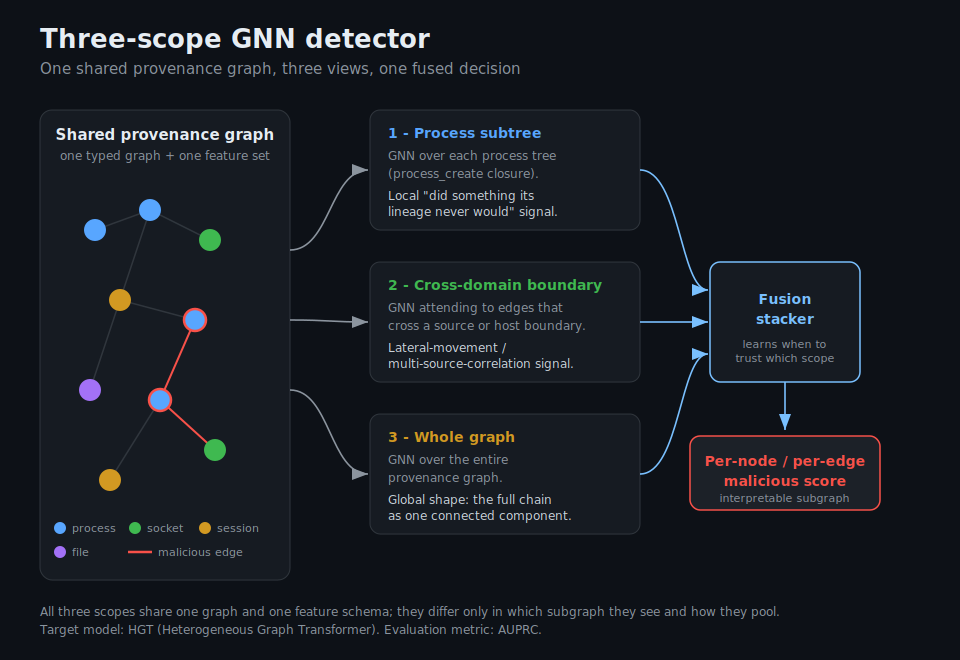
The goal in this project isn’t a single network. It’s three! Each one looking at the same graph through three different windows, with a fourth model learning how to combine them. The research I referenced earlier looked at entirely different aspect of a Graph. I’m hoping by combining multiple views into one the whole will be more than the sum of its parts.

Scope one: the process subtree. A GNN passed over each process tree. This is the scope that catches “this process did something its own lineage would never do.” The credential dump, viewed inside the subtree of the session that spawned it, is anomalous against its siblings and parents. Here we have only the local context, and only the local anomaly.
Scope two: the cross-domain boundary. A GNN that specifically attends to edges crossing a boundary. For example a host boundary (the RDP hop from workstation to DC). This is the lateral-movement scope. It exists because the events that exhibit lateral movement are exactly the ones a single-source tool structurally cannot correlate. Boundary-crossing events are a signal, so a scope dedicated to boundary edges should see it most clearly.
Scope three: the whole graph. A GNN over the entire provenance graph, to catch the global shape. The full chain as one connected component, the thing you only see when you zoom all the way out.

alt text (Area Under the Precision-Recall Curve)

The important design constraint: all three scopes share one graph and one set of features. They differ in which subgraph they see but not in what a node’s feature vector contains. That’s what kept the feature work tractable. I built one schema to serve all three, rather than three schemas.

So why ~~male models~~ GNNs? My Intuition is that a single model over the entire provenance graph faces a resolution problem: the malicious subgraph is a handful of nodes and edges inside thousands. The signals that can identify it live at varying scales.

The credential dump is a local anomaly, a process doing something its immediate lineage would not normally exhibit. A whole-graph model, containing information across thousands of nodes, tends to wash that sort of fine detail out.
The lateral movement is the opposite: its signal is precisely that an edge crosses a boundary between log sources or between hosts, which is easy to miss unless you’re specifically attending to boundary-crossing edges rather than treating them like any other connection.
The overall shape of the attack and the fact that these scattered events form one long connected chain. This picture can only resolve when you zoom all the way out. No single receptive field is right for all three.

Models tend to be tuned and focused on a single thing it’s designed for. A model tuned to catch the local anomaly blurs the global structure; a model tuned for global structure misses the local detail. So instead of forcing one network to compromise across all three scales, each scope is specialised for the signal it’s best placed to see. Then we can introduce a fusion model learns when to trust each individual model. This whole premise is built on my intuition that the three are good at different aspects of identifying maliciousness and a stacker can arbitrate between them better than a single averaged view can. Whether that intuition holds up you’ll have to wait until the results come out in part 2!

If an analogy would be helpful; think of it like photographing a crime scene at three settings. Zoom right in and you can see one suspicious detail in sharp focus, but you’ve lost all sense of where it sits or what it connects to. Pull all the way back and you can see the whole scene as one shape, every element and how they’re arranged, but the incriminating detail is now too small to make out.

The third setting isn’t really a zoom at all: it’s a filter that lights up only the doorways and boundaries, the points where someone moved from one room, or one building, to another. I this kind of attack, the act of crossing that boundary is the tell. None of the three is the “right” setting. Each shows what the others can’t. The difference from a camera is that we don’t pick the best shot, we use all three to form a narrative of who done it.

Sounds great in theory but..

Everything I’ve described so far assumes I have data, like lots and lots of data. Well labelled, multi-source telemetry that is capable of capturing the details of a multi-stage attack. With known ground truth of what happened and why so we can train and test against using supervised learning. Most importantly data that looks enough like the real thing to train on. This is arguably the biggest blocker and hardest part of any machine learning project.

The options for getting attack telemetry are all bad in different ways. Real production logs are a compliance and privacy minefield. The well-known public datasets (LANL, DARPA OpTC) have been scrubbed and anonymised to the point where they read more like generic event abstractions than actual log sources. Which unfortunately strips out exactly the cross-source detail a correlation-based detector needs.

You can generate your own with attack-simulation frameworks like Atomic Red Team or Caldera, but that needs real a lot of well maintained infrastructure to run against. Which takes time and resources and unfortunately scales poorly when what you need breadth in your datasets. Most off-the-shelf synthetic log generators have flaws for this use case, the biggest one being: they emit each log format independently. So the records don’t agree with each other, two sources will disagree about a port number or a timestamp, which is the number-one tell of fake data. This completely destroys any causal consistency the whole approach of using GNNs depends on.

Thankfully it looks like Cisco’s EvidenceForge is what changed that,it’s an open-source tool from Cisco Talos that was released only weeks before I wrote this. Its whole design premise is the problem above. Instead of generating each log format separately, it works from a single canonical event model. One source of truth for every event and emits all the different log formats from that same object. Two emitters physically cannot disagree about a port, a timestamp, or a logon ID, because there’s only one underlying value, fantastic! On top of that it enforces causal and temporal ordering (the dependencies that have to hold in reality. For example a DNS lookup occurs before the HTTPS connection is resolved. A Kerberos ticket before the domain logon they enable), layers in realistic background noise and red herrings so the malicious activity isn’t trivially separable, and models believable timing rather than the uniform-random timestamps.

What it produces, concretely, is a synchronised dataset across 20-plus correlated log formats. Windows Security events, Sysmon, many Zeek log types, eCAR EDR/XDR telemetry, and more. All unified in describing the same scenario, all agreeing with each other, all with known “ground-truth” labels which is key for supervised learning. For this project I use four of those formats (eCAR, Windows Security, Sysmon, Zeek). The scenario authoring is LLM-assisted, you provide a description of the attack you want and it builds the canonical event. However importantly, the generation itself is entirely deterministic, so a scenario is reproducible. That combination of realistic and varied but reproducible and labelled, is exactly what a project like this needs and exactly what didn’t exist a couple of months ago.

So when I talk about “a scenario” in this post, that’s what’s underneath it: an EvidenceForge generated, causally consistent, ground truth labelled multi source capture. The project is, in a real sense, only achievable because that tool now exists.

The Data Pipeline: parse, correlate, label

Before any of the GNN ambition, you need the graph. And the graph has to be correct, which is a much higher bar than “the code runs.” A graph that’s subtly wrong, for example an edge anchored to the wrong entity or a label on the wrong node will train a model that learns the wrong thing and reports a great-looking accuracy number while doing so. In essence the data pipeline is the project.

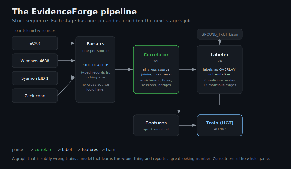
The pipeline is a strict sequence: parse -> correlate -> label -> features -> train. Each stage has one job and I’ve taken pains to enforce it doesn’t encroach on next stage’s job. The reasoning behind this is every Machine Learning project I’ve attempted has taught me that being able to be flexible, iterate and modify process is key to getting a good output. If we were to combine everything into a monolith it means making targeting tweaks much more fragile and frankly it can be hard to find where you’ve scurried away different functions. That discipline mattered more than I expected, so let me go through the first three.

Parsers are pure readers

Each source gets its own parser: ecar.py, windows.py, sysmon.py, zeek.py. A parser reads its source into typed records and does nothing else. No cross-source logic, no correlation, no clever joins. The moment a parser starts reaching into another source’s data to “help,” you’ve created a place where a correlation bug can hide that no correlation test will catch, because it’s happening in the parser.

The correlator does all the joining

correlator.py (currently on its ninth version… the version numbers tell their own story) is where the four sources become one graph. Needless to say this is the hard part.

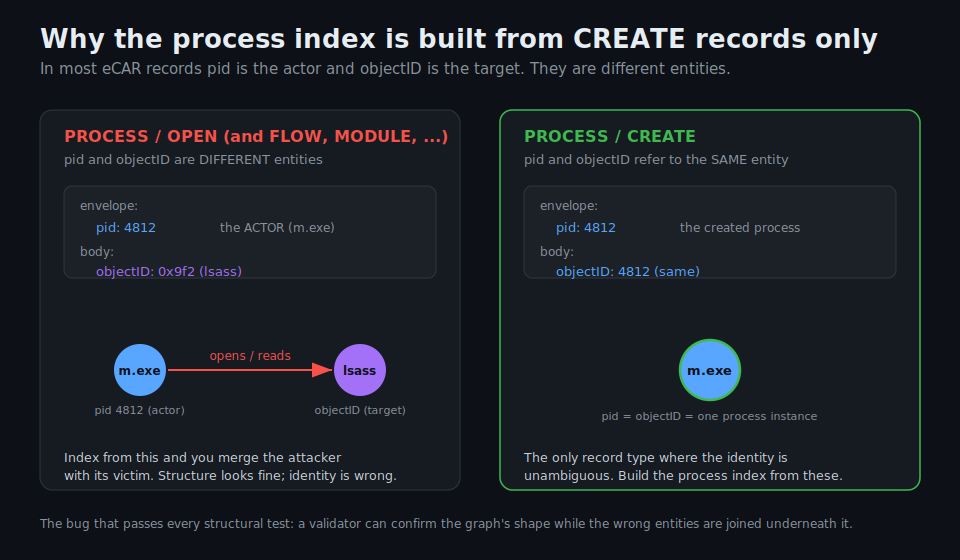
The join that builds the process graph relies on matching process identity across eCAR’s record types. eCAR has multiple action types: PROCESS/CREATE, OPEN, FLOW, MODULE, to name a few. Each carries a pid and an objectID. The naive move is to index processes from any record that mentions them. That is wrong, and why it’s wrong subtle: in most record types the pid is the “actor” (the process doing the thing) while the objectID is the target (the process being acted upon). They’re different entities. Only in PROCESS/CREATE records do the envelope pid and the objectID reliably refer to the same process. So the process-instance index has to be built exclusively from CREATE records. Build it from anything else and you’ll happily merge an attacker process with its victim because they appeared in the same OPEN record, and every structural test will still pass because the structure is fine. It’s the identity that’s wrong.

alt text

The correlator also does the cross-source enrichment (joining eCAR processes to their Windows/Sysmon counterparts to recover fields eCAR lacks, like logon_id), the network-flow merge (Zeek conns). Session stitching is where I’ve built the socket-to-session bridge that connect a network flow to the session that owns it. Those bridges are what allows us to see the RDP hop as a single correlated thing rather than two unconnected halves. They’re built in the correlator.

The labeler is an overlay, not a mutation

labeler.py (on v4, again the versions are their own story) takes the built graph plus a ‘ground-truth’ file and marks which nodes and edges are malicious. One decision here paid off: the labels are an overlay, not a mutation of the graph. The graph is one object, the labels are a separate dataset set that references it. This means I can rebuild labels without rebuilding the graph, diff label versions against a fixed graph, and crucially keep the graph as the independent artifact it should be.

The labelling result on the first scenario I built with Evidence Forge. Six malicious nodes, thirteen malicious edges, against a graph of 3,111 nodes and 2,106 edges. Ruminate on that for a moment, because they’re the entire challenge for the back half of this project. The malicious nodes are 0.19% of nodes and the malicious edges are 0.62% of edges. This is the kind of realism running Adversary Simulation against an attack range struggles with. The events associated with a real attack are a rounding error against background enterprise activity.

alt text

Where this actually is right now

So I ran the first training pass: a deliberately minimal HGT over the whole graph, no held-out data, trained on everything. It fit. Loss fell cleanly, the edge-level AUPRC (Area Under the Precision-Recall Curve) climbed to a perfect 1.0, every integrity check passed.

To be clear though in reality that 1.0 is worth nothing, and that’s exactly the output I wanted to see. The model was shown all thirteen malicious edges with the entire graph visible and no test set held back. A perfect score there means one thing: the plumbing works end to end, the artifact loads, the graph feeds the model, gradients flow through every relation type, the loss does what a loss should. All it’s proven is that the model can memorise thirteen edges it was handed the answers to.

You may be pondering that a perfect score that proves nothing is a strange thing to be happy about. If we were to think about the alternative it would be the loss falling while the model quietly learned to predict “benign” for everything. It didn’t happen; the model actually found the positives.

One genuinely useful thing did fall out of that run. The malicious persistence service node has no edges. None! So in the current graph it isn’t connected to anything structurally it’s invisible. Meaning no graph model can learn it from a node that floats unconnected. Not a model bug, but it’s a gap in how the graph encodes that particular step, and it goes on the list for the feature stage to fix upstream. I found it because the model tried to use the graph and the graph came up short.

Next Steps & Ambitions

Besides some minor tweaks such as the aforementioned edgeless service we’ve hit a limit with what the simple scenario I produced can do. If you’re thinking right now—and congrats on reading this far—that conducting a supervised ML project on a single scenario is nonsensical, you are right. I’ll need to create many more complex scenarios to properly form a training and test dataset. Another missing puzzle piece is temporal. Currently the timestamp is not being captured in my Graph which is key context the Model is currently lacking. Finally i’ll be A B testing with the 3 layer GNN vs a single GNN.

To be blunt I can see this taking a while as this is work being conducted in my free time among a bunch of other projects which are at varying stages and likely will never see the light of day. But I’m keen as soon as I have anything tangible to share both in terms of results and the whole codebase it will be provided on my GitHub.